When people say:

“I used machine learning to predict the price using linear regression.”

it can sound more complicated than it actually is.

There may be a lot of terminology around machine learning, models, training, parameters, and predictions. But if we strip away the terminology, simple linear regression is fundamentally a mathematical problem.

At its core, we are trying to find just two numbers:

• The intercept — $\beta_0$
• The slope — $\beta_1$

Once we have those two numbers, making a prediction is simply a matter of putting a value into an equation.

1. The basic idea

Suppose we want to predict someone’s salary based on their years of experience.

We have some historical data:

We can plot these observations on a graph.

Scatter plot of salary versus years of experience with the fitted regression line

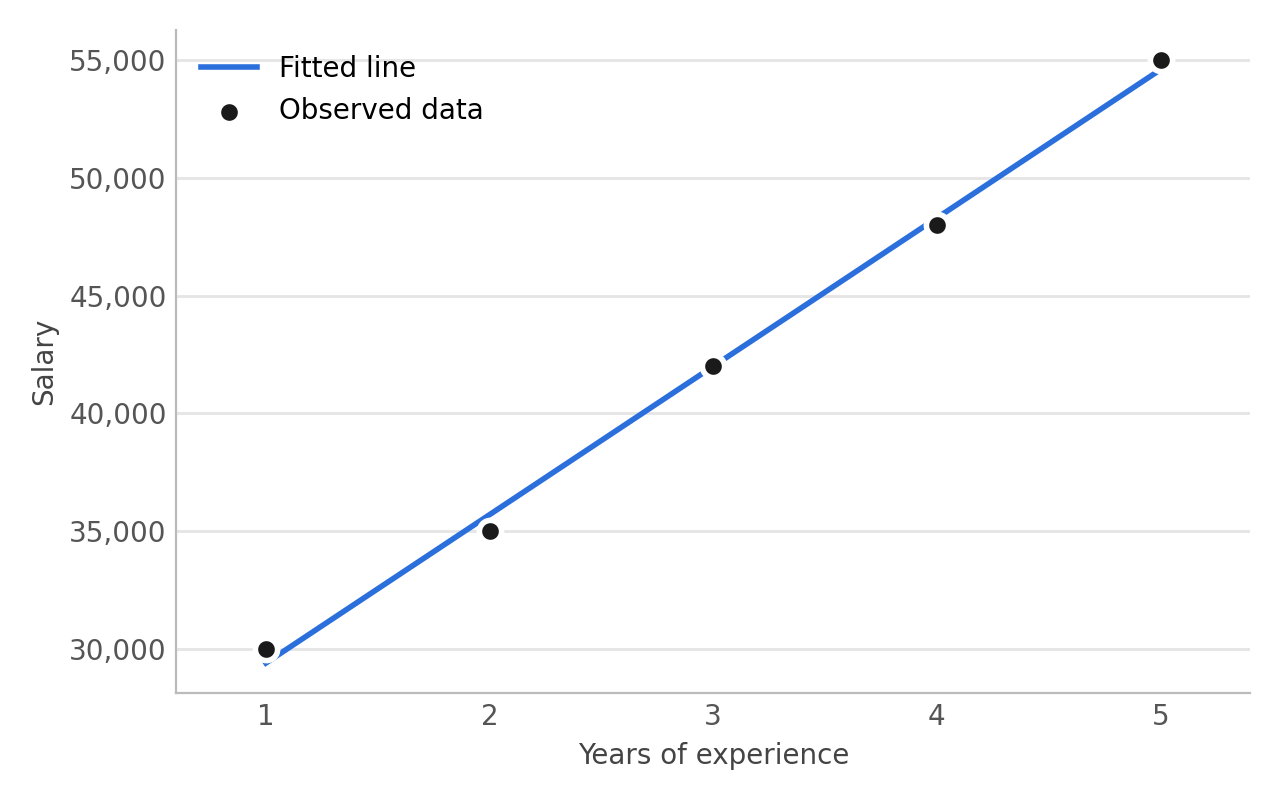
The goal of linear regression is to find a straight line that represents the relationship between experience and salary.

The equation of that line is:

$\hat{y} = \beta_0 + \beta_1 x$

Where:

• $\hat{y}$ = predicted value
• $x$ = input value
• $\beta_0$ = intercept
• $\beta_1$ = slope

That’s essentially our entire prediction model.

2. What does the slope mean?

The slope tells us how much the predicted output changes when the input increases by one unit.

For example, suppose we calculate:

$\beta_1 = 5{,}000$

This means that for every additional year of experience, the predicted salary increases by approximately $5,000.

So if our model is:

$\hat{y} = 25{,}000 + 5{,}000x$

then:

• 1 year → $30,000
• 2 years → $35,000
• 3 years → $40,000
• 4 years → $45,000

The slope controls how steep the line is.

3. What does the intercept mean?

The intercept is the predicted value of $y$ when $x=0$.

Suppose:

$\beta_0 = 25{,}000$

Then our model says:

$\hat{y} = 25{,}000 + 5{,}000x$

When experience is zero:

$\hat{y} = 25{,}000 + 5{,}000(0)$

Therefore:

$\hat{y} = 25{,}000$

So the intercept is:

The point where the regression line crosses the $y$-axis.

Depending on the problem, the intercept may or may not have a meaningful real-world interpretation. Mathematically, however, it is one of the two parameters needed to define the line.

4. So where do the slope and intercept come from?

This is where the interesting mathematics happens.

We don’t simply guess:

$\beta_0 = 25{,}000$

and

$\beta_1 = 5{,}000$

Instead, we calculate values that produce the best-fitting line for the observed data.

One common approach is called Ordinary Least Squares (OLS).

The idea behind OLS is simple:

Find the line that minimizes the total squared difference between the actual values and the predicted values.

For each observation, we have an error:

$e_i = y_i - \hat{y_i}$

Since some errors are positive and others are negative, simply adding them together could cause them to cancel each other out.

Instead, we square each error.

The objective becomes:

$\text{SSE} = \sum_{i=1}^{n} (y_i - \hat{y}_i)^2$

Since:

$\hat{y_i} = \beta_0+\beta_1x_i$

we can write:

$\text{SSE} = \sum_{i=1}^{n} \left( y_i - \beta_0 - \beta_1 x_i \right)^2$

OLS finds the values of $\beta_0$ and $\beta_1$ that minimize this quantity.

5. Deriving $\beta_0$ and $\beta_1$ using partial derivatives

We have already defined the Sum of Squared Errors:

Our goal is to find the values of $\beta_0$ and $\beta_1$ that make this SSE as small as possible.

Because we have two unknowns, $\beta_0$ and $\beta_1$, we take the partial derivative with respect to each one.

Step 1: Find $\beta_0$

Start with:

We differentiate with respect to $\beta_0$:

The summation can remain outside:

Now we use the chain rule. If:

then:

Since:

we get:

At the minimum SSE, the derivative must be zero: $2 \sum_{i=1}^{n} \left(y_i - \beta_0 - \beta_1 x_i\right) = 0$

Divide by $-2$:

Expand the summation:

Because $\beta_0$ and $\beta_1$ are constants:

Rearrange:

Divide by $n$:

But:

and:

Therefore:

So this is where the intercept formula comes from.

Step 2: Find $\beta_1$

Now we differentiate the same SSE with respect to $\beta_1$:

Again, using the chain rule, the derivative of the inside is:

Therefore:

At the minimum: $2 \sum_{i=1}^{n} x_i \left(y_i - \beta_0 - \beta_1 x_i\right) = 0$

Divide by $-2$:

Expand:

Therefore:

Now we already know that:

Substitute this into the equation:

Since:

we get:

Expand:

Move $n\bar{x}\bar{y}$ to the left:

Therefore:

This can be rewritten using deviations from the mean:

This is the familiar OLS slope formula.

Setting the derivatives to zero only finds a stationary point, but here it is the minimum: SSE is a convex function of $\beta_0$ and $\beta_1$ (a sum of squared linear terms), so its only stationary point is the global minimum.

6. The whole idea in one flow

So the entire process is:

Specifically:

Then:

Differentiate with respect to $\beta_0$:

which gives:

Differentiate with respect to $\beta_1$:

which gives:

Therefore, linear regression is not simply guessing a line.

It uses calculus to find the values of $\beta_0$ and $\beta_1$ that produce the minimum possible squared error for the training data.

5. Calculating the slope

For simple linear regression, the optimal slope is:

At first, this formula can look intimidating. Let’s break it down.

$\beta_1$

This is the slope of our regression line.

$x_i$

This represents an individual observed input value.

For example, if our input is years of experience:

could represent an employee with 3 years of experience.

$y_i$

This represents the corresponding observed output.

For example:

could be that employee’s actual salary.

$\bar{x}$ and $\bar{y}$

$\bar{x}$ — This is the mean of all the input values:

$\bar{y}$ — This is the mean of all the output values:

Numerator

The numerator is:

It measures how $x$ and $y$ vary together around their respective means.

• If larger values of $x$ generally occur with larger values of $y$, this quantity tends to be positive.
• If larger values of $x$ generally occur with smaller values of $y$, it tends to be negative.

Denominator

The denominator is:

This measures how much the input $x$ varies around its mean.

So, conceptually, the slope can be thought of as:

Calculating the intercept

Once we have calculated the slope, the intercept is much simpler. The formula is:

Again, let’s understand the terms:

• $\beta_0$ = intercept
• $\bar{y}$ = mean of the target values
• $\beta_1$ = calculated slope
• $\bar{x}$ = mean of the input values

So the process is essentially:

Once we have $\beta_0$ and $\beta_1$, our model is ready.

7. Now prediction becomes extremely simple

Suppose our calculations give us:

and:

Our model becomes:

Now suppose someone has 6 years of experience.

We simply substitute:

Therefore:

That’s the prediction.

There is no mysterious “AI thinking” happening here.

The model has learned two numbers:

and

Then it applies the equation.

8. So what does model.fit(X, y) actually do?

This is where the machine-learning terminology can make things sound more complicated than they are.

In Python, we might write:

from sklearn.linear_model import LinearRegression

model = LinearRegression()

model.fit(X, y)

When we call:

model.fit(X, y)

we are essentially asking the algorithm:

“Look at these examples and find the parameters that give the best-fitting linear relationship.”

For simple linear regression, those parameters are:

$\beta_0$

and

$\beta_1$

After fitting the model, we can inspect them:

print(model.intercept_)
print(model.coef_)

Conceptually:

model.fit(X, y)

        ↓

Find β₀ and β₁

        ↓

ŷ = β₀ + β₁x

        ↓

Use the equation for prediction

Scikit-learn uses numerical linear-algebra methods internally rather than necessarily evaluating the formulas above literally step by step. But mathematically, for ordinary simple linear regression with an intercept, it is solving the same least-squares problem.

9. Why do we call this “Machine Learning”?

This is perhaps the most interesting part.

The mathematics itself is not new.

Linear regression has a long history in statistics and mathematics.

What makes it part of a machine-learning workflow is the idea that:

1. We provide data.
2. An algorithm estimates parameters from that data.
3. The resulting model is used to make predictions on new data.

For linear regression, the learned parameters happen to be:

$\beta_0,\quad\beta_1$

For more complicated machine-learning models, there may be thousands, millions, or even billions of parameters.

But the basic idea remains:

Use data to estimate parameters, then use those parameters to produce predictions.

10. The important mental model

When you hear:

“I trained a linear regression model.”

don’t imagine a mysterious black box.

For simple linear regression, imagine this:

                 Training Data
                      │
                      ▼
             Find the best β₀, β₁
                      │
                      ▼
              ŷ = β₀ + β₁x
                      │
                      ▼
                 New input x
                      │
                      ▼
                  Prediction ŷ

The “learning” part is essentially finding the parameters.

The “prediction” part is simply using those parameters in the equation.

11. The bigger picture

Linear regression is a beautiful example because it lets us see what is happening underneath the machine-learning terminology.

At the surface, we might write:

model.fit(X, y)

and:

model.predict(X_new)

But underneath those convenient APIs is mathematics.

The fundamental process is:

$\boxed{\ \text{Data}\ \rightarrow\ \text{Optimization}\ \rightarrow\ \text{Parameters}\ \rightarrow\ \text{Prediction}\ }$

For simple linear regression:

$\boxed{\ \text{Optimization}\ \rightarrow\ \beta_0,\beta_1\ }$

and then:

$\boxed{\ \hat{y}=\beta_0+\beta_1x\ }$

That’s really what is happening behind the scenes.

Final takeaway

The next time someone says:

“I used machine learning to predict something using linear regression.”

remember what is actually happening.

There is a dataset.

We find the line that best fits the data using a mathematical optimization method such as Ordinary Least Squares.

That gives us two important parameters:

$\boxed{\beta_1 = \frac{\sum_{i=1}^{n}(x_i-\bar{x})(y_i-\bar{y})}{\sum_{i=1}^{n}(x_i-\bar{x})^2}}$

and:

$\boxed{\ \beta_0=\bar{y}-\beta_1\bar{x}\ }$

Then we put them into:

$\boxed{\ \hat{y}=\beta_0+\beta_1x\ }$

And that’s the prediction.

The “machine learning” label doesn’t make the mathematics disappear. In this case, the machine is essentially helping us estimate the parameters from data. The prediction itself is just the equation.